Time spent: 4h
Total: 9.5h/10000h
Integrals are probably going to be the last thing I’ll cover in calculus in a while. I will probably come back to look into partial derivatives at some point.
The integral is a great tool for calculating areas. It is also defined as a limit, just like its’ counterpart - the derivative. Before looking into the formal definition, let’s first ask a question: how can one calculate the area under a curve of a function?
Now, the answer to this question is actually a bit trickier. There really is no good way to calculate the exact area; one can really just approximate it. Here’s an approach on how one might do so.
Consider the function over the interval . It looks like this:
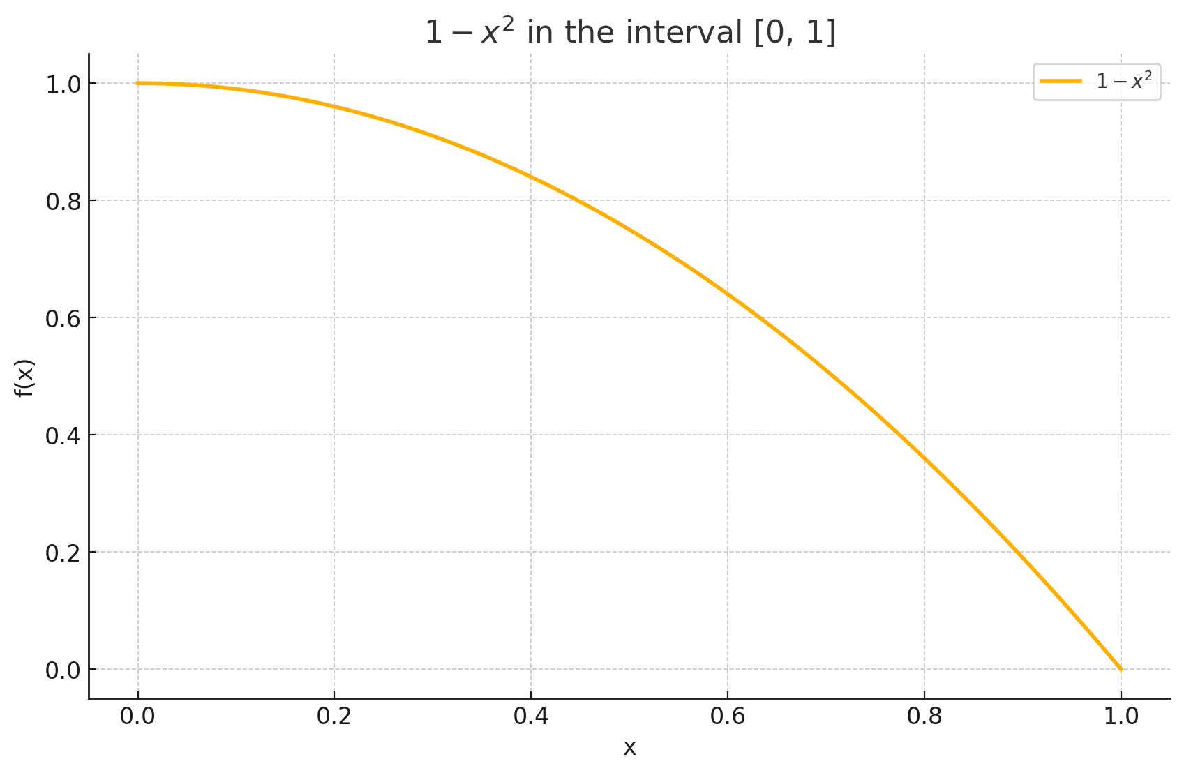
Graphic of f(x). (Source: ChatGPT/matplotlib)
The way to approximate the area would be to draw rectangles under the curve. The rectangles would be of height and of a width that can be decided based on , the number of rectangles we want to draw. Let’s try this with :
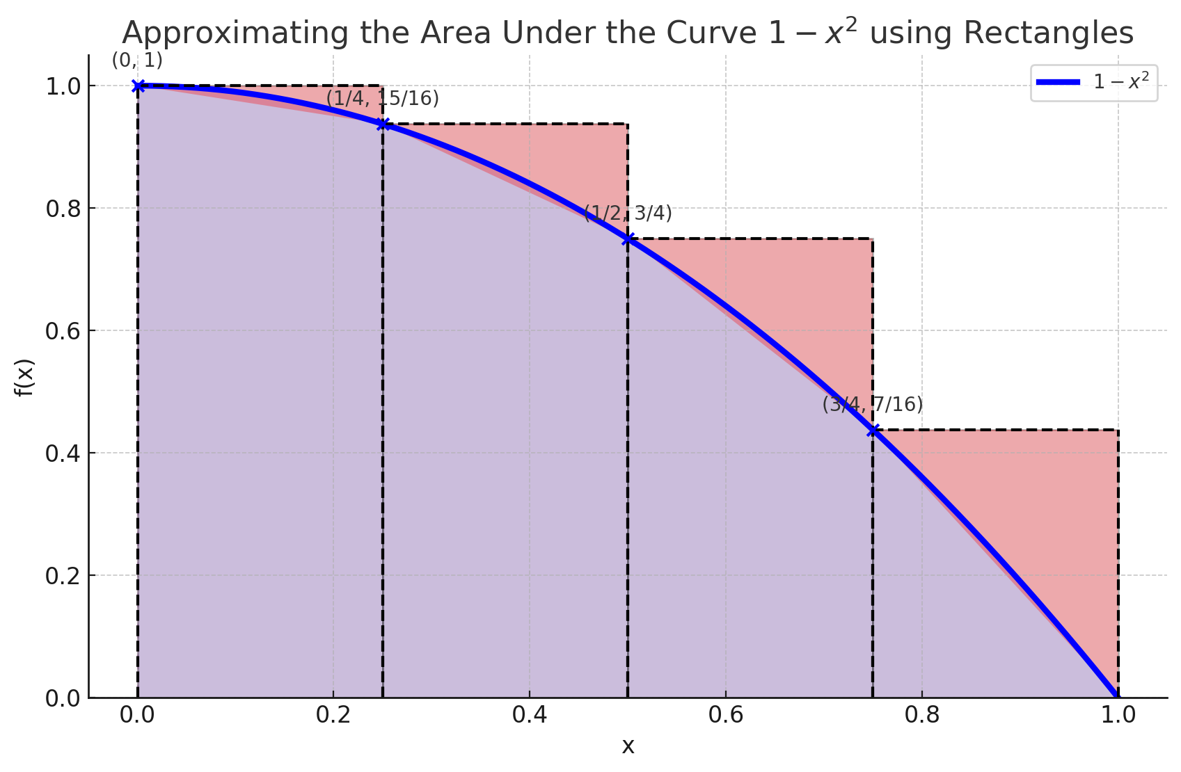
Graphic of f(x) with 4 rectangles approximating the area. (Source: ChatGPT/matplotlib)
Ugh. Seems like quite a rough approximation, doesn’t it? It does overshoot quite a bit. This is called the upper sum of . The upper sum uses the point of the maximum value of in the subinterval the rectangle forms.
Here the width of the rectangles is 1/4. Let’s consider that as . The calculation for the sum would simply be
What if one used the point of the minimum value of in the rectangle (also known as the partition P)‘s subinterval? That’s when you get what’s called a lower sum. Here’s a graphical illustration of that too:
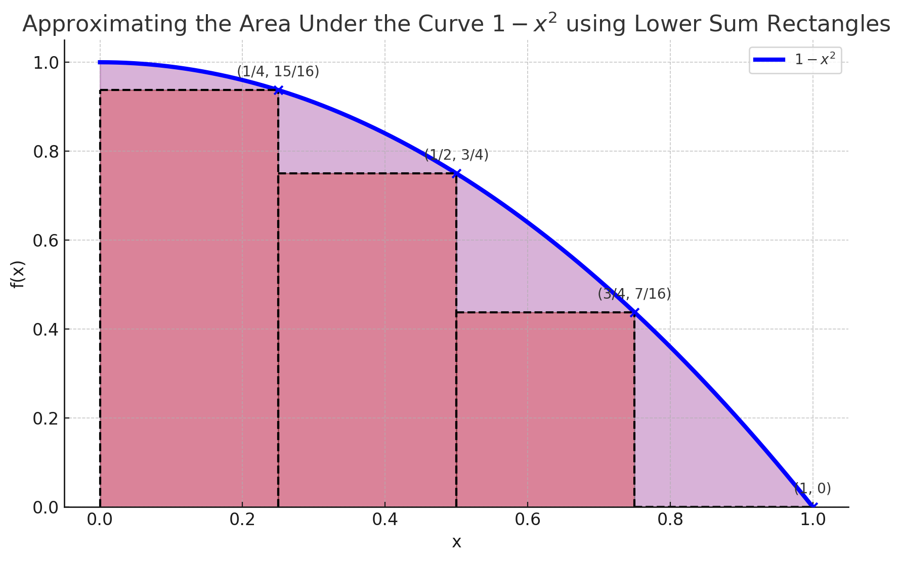
Graphic of f(x) with 4 rectangles approximating the lower sum. (Source: ChatGPT/matplotlib)
Now the calculation would go like this:
Another way of approximating the area is what’s called the midpoint rule. The midpoint rule uses the midpoint of each rectangle, as opposed to the maximum or the minimum value. The area approximation given by the midpoint rule is always between the lower and the upper sums. See:
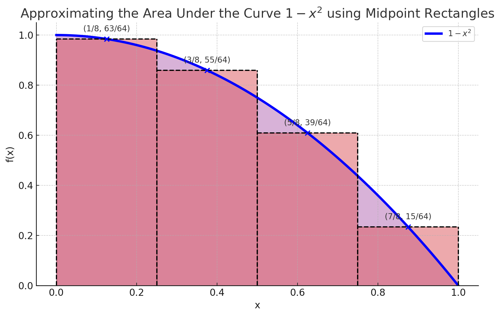
Graphic of f(x) with 4 rectangles approximating the midpoint sum. (Source: ChatGPT/matplotlib)
The midpoint approximation is often the most precise. The calculation follows the same principle:
The precision of all of these approximations will improve as the amount of rectangles () increases. Let’s try instead:
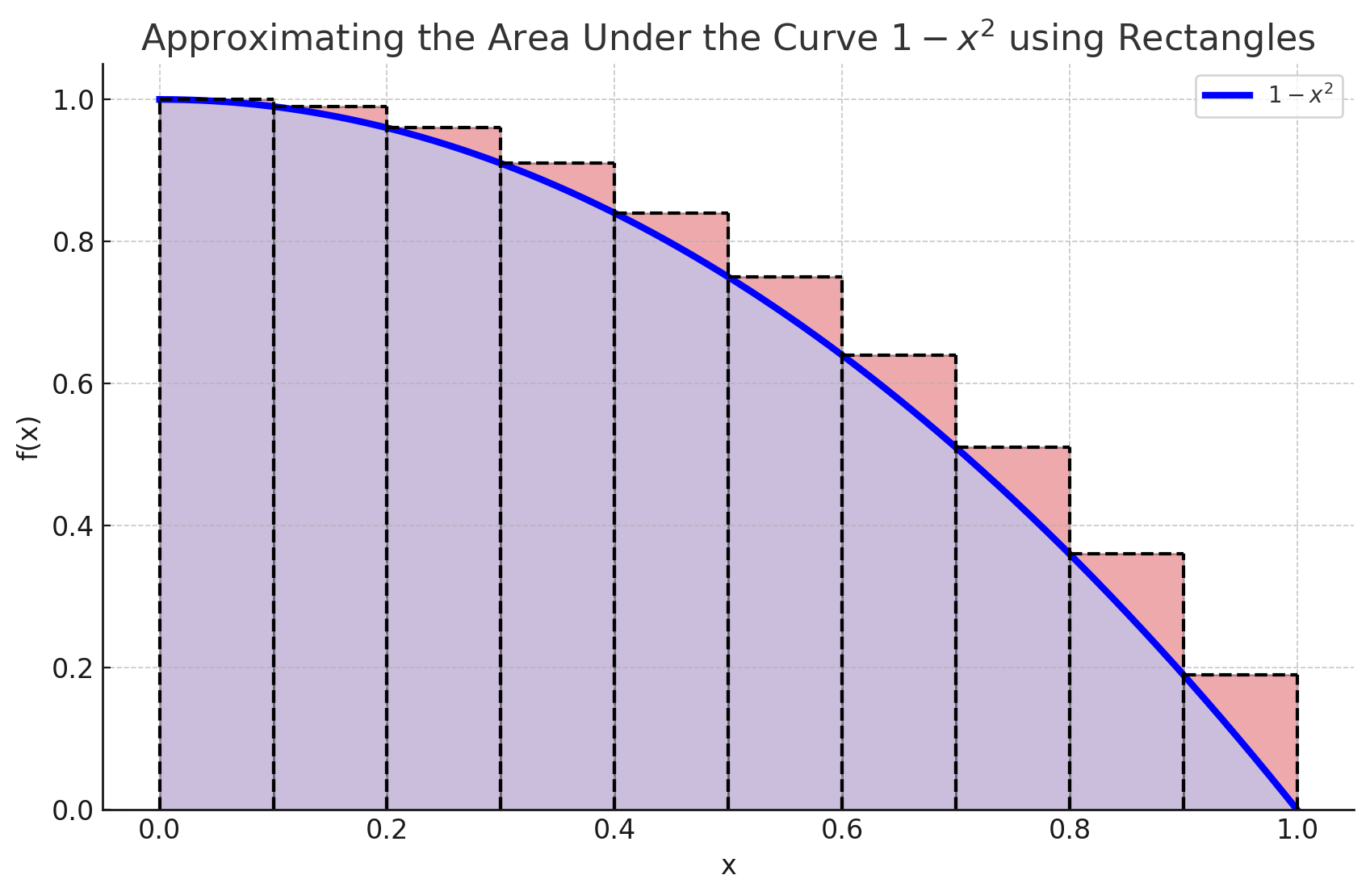
Graphic of f(x) with 10 rectangles approximating the upper sum. (Source: ChatGPT/matplotlib)
That’s better. The approximation is still a bit rough though. But that’s fine. This is only to illustrate the principle. Let’s try doing this in Python to save the job of calculating these manually.
import numpy as np

def f(x):
    return 1 - x ** 2

lower_bound = 0
upper_bound = 1

# n = amount of rectangles
def lower_sum(n):
    rectangle_width = (upper_bound - lower_bound) / n

    S = 0

    for i in range(n):
        # all the x values in the rectangle (also known as the partition P)
        x_i = np.linspace(i * rectangle_width, (i + 1) * rectangle_width)

        # the lowest value of f(x) in x_i
        m_i = np.min(f(x_i))

        S += m_i * rectangle_width

    return S

def upper_sum(n):
    rectangle_width = (upper_bound - lower_bound) / n

    S = 0

    for i in range(n):
        # all the x values in the rectangle (also known as the partition P)
        x_i = np.linspace(i * rectangle_width, (i + 1) * rectangle_width)

        # the highest value of f(x) in x_i
        m_i = np.max(f(x_i))

        S += m_i * rectangle_width

    return S

def midpoint_sum(n):
    rectangle_width = (upper_bound - lower_bound) / n

    S = 0

    for i in range(n):
        x_i = (i * rectangle_width + (i + 1) * rectangle_width) / 2

        # the highest value of f(x) in x_i
        m_i = np.max(f(x_i))

        S += m_i * rectangle_width

    return S
Testing these functions with should yield the same results.
> print(lower_sum(4))
0.53125

> print(upper_sum(4))
0.78125

> print(midpoint_sum(4))
0.671875
Nice! Let’s make a table of the approximations the program gives when goes up.
| lower_sum | midpoint_sum | upper_sum | |
|---|---|---|---|
| 4 | 0.53125 | 0.67125 | 0.78125 |
| 25 | 0.6464 | 0.6668000000000001 | 0.6864 |
| 50 | 0.6565999999999999 | 0.6667 | 0.6765999999999999 |
| 100 | 0.6616500000000002 | 0.6666749999999999 | 0.6667166649999995 |
Seems like the values are all approaching . If , all of the values would equal exactly that.
What we saw is called the Riemann sum on the interval . It is formally defined as:
where , the partition, is the set of some points on the interval .
Definite Integrals
We can extend the Riemann sum a bit - the Riemann integral is formally defined as the limit:
Where:
- is the notation for a definite integral.
- is the width of the subinterval (the rectangle).
- is some point on the graph of .
However, calculating the values of definite integrals is a bit inconvenient using the Riemann sums. Another approach is to use antiderivatives. The antiderivative of a function is defined when .
The Fundamental Theorem of Calculus states that if is continuous on the interval , and is any antiderivative of on , then
This gives us a method to solve definite integrals without having to calculate the limits of Riemann sums. We only need to:
- Find an antiderivative of , and
- Calculate the value .
When solving antiderivatives, you just have to think backwards.
Example 1: Evaluate .
Solution:
- For what value is the derivative? It can be rewritten as , and we know from the power rule () that the antiderivative must be .
- For what value is - the derivative? We know that , so the antiderivative must be .
- So we have the antiderivative, which is . We need to evaluate it at and to find the definite integral.
Cool! Let’s try evaluating the definite integral we were looking at before.
Example 2: Evaluate .
Solution: The antiderivative of is .
Looks like our approximations were correct.
Indefinite Integrals & Solving by Substitution
The indefinite integral is defined as the set of all antiderivatives of . Since antiderivatives only differ by a constant C, for any antiderivative we have:
Substitution Method
The substitution method is also just about thinking backwards. For example, we know from the chain rule that is . We can look at it from another perspective and say that .
Example 1: Find
Solution:
- Consider . Let’s rewrite the integral as . This integral does not fit the formula , (since ) so let’s rewrite more.
- Rewrite the integral as .
- Now we have . Integrate that and get .
- Substitute for and get .
That’s enough for integrals. I used Thomas’ Calculus, Early Transcendentals - 15th edition as my resource for studying. Most definitely gonna also check out other resources like 3Blue1Brown when I need to gain a deeper understanding.
I found some exercises for (indefinite) integrals here.