The Start of The Linear Algebra Grind - Day 7 of ML

Time spent: 2h
Total: 18h/10000h

I’m gonna be doing a LOT of linear algebra now. I have a great book for it - Gilbert Strang’s Linear Algebra and Its Applications. Don’t expect much but linear algebra in the upcoming days… or weeks.

Let’s get straight to the point. The central problem of linear algebra is solving linear equations. We’ll later be looking at numeric and algorithmic ways to solve them, but let’s first take a look at some graphical methods.

Visualizing Linear Equations

Let’s first consider a very easy example - one that could easily be solved without any knowledge of linear algebra.

Consider these two equations:

We can take a look at this system in terms of rows or columns.

Let’s first take a look at the row variant. Each one of the rows forms a line. And the intersection of these lines is the solution to the system. Seems trivial enough:

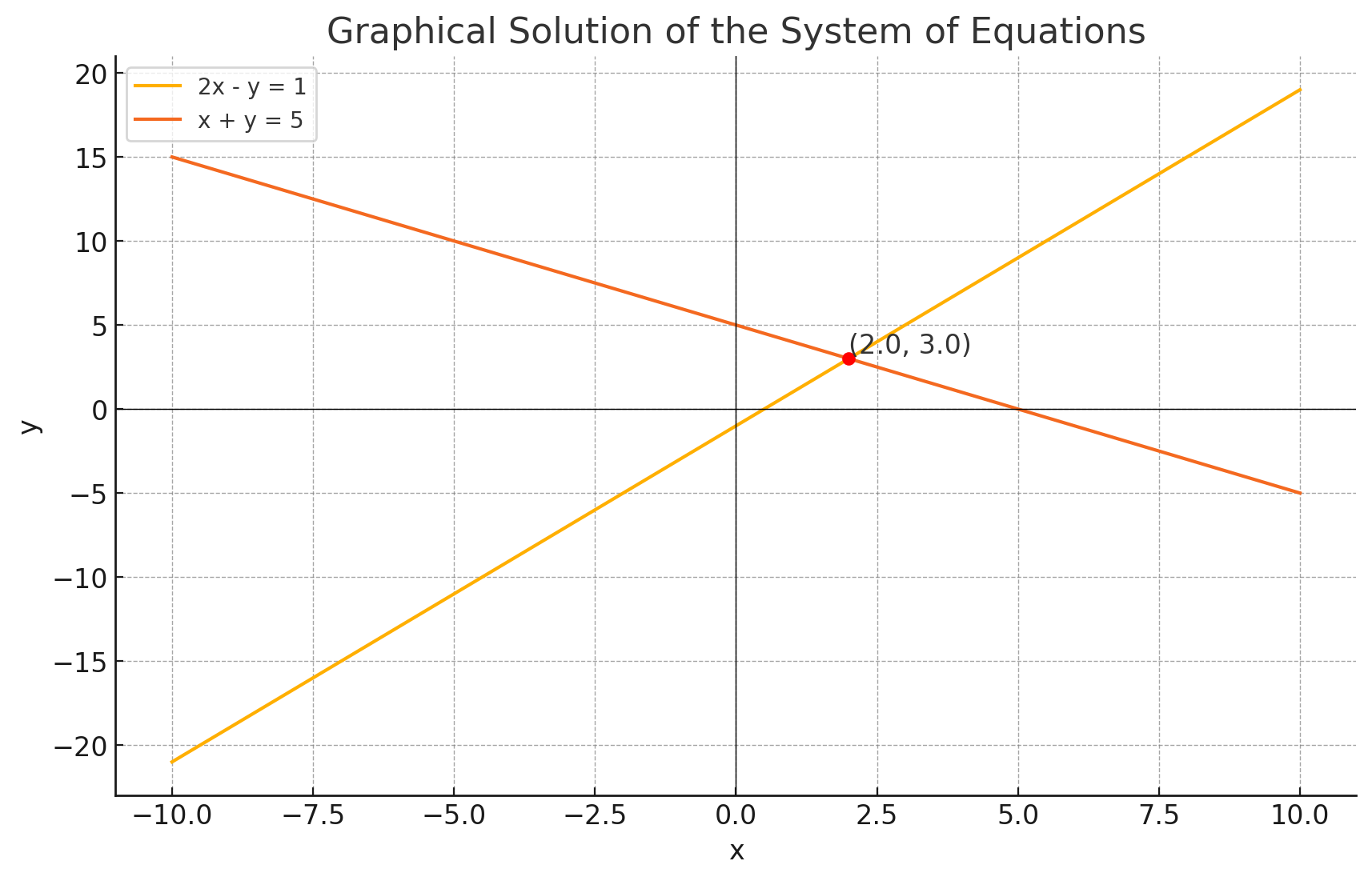
Solution to the system using lines. (Source: ChatGPT/matplotlib)

And it is indeed trivial. The solution is $\{x=2, y=3\}$.

Let’s try viewing this in terms of columns. The column form for this system is

So the first column vector is $\begin{bmatrix} 2 \\ 1 \\ \end{bmatrix}$ and the second one is $\begin{bmatrix} -1 \\ 1 \\ \end{bmatrix}$. Here we have to solve for the unknown coefficients $x$ and $y$. Let’s see how this plays out graphically:

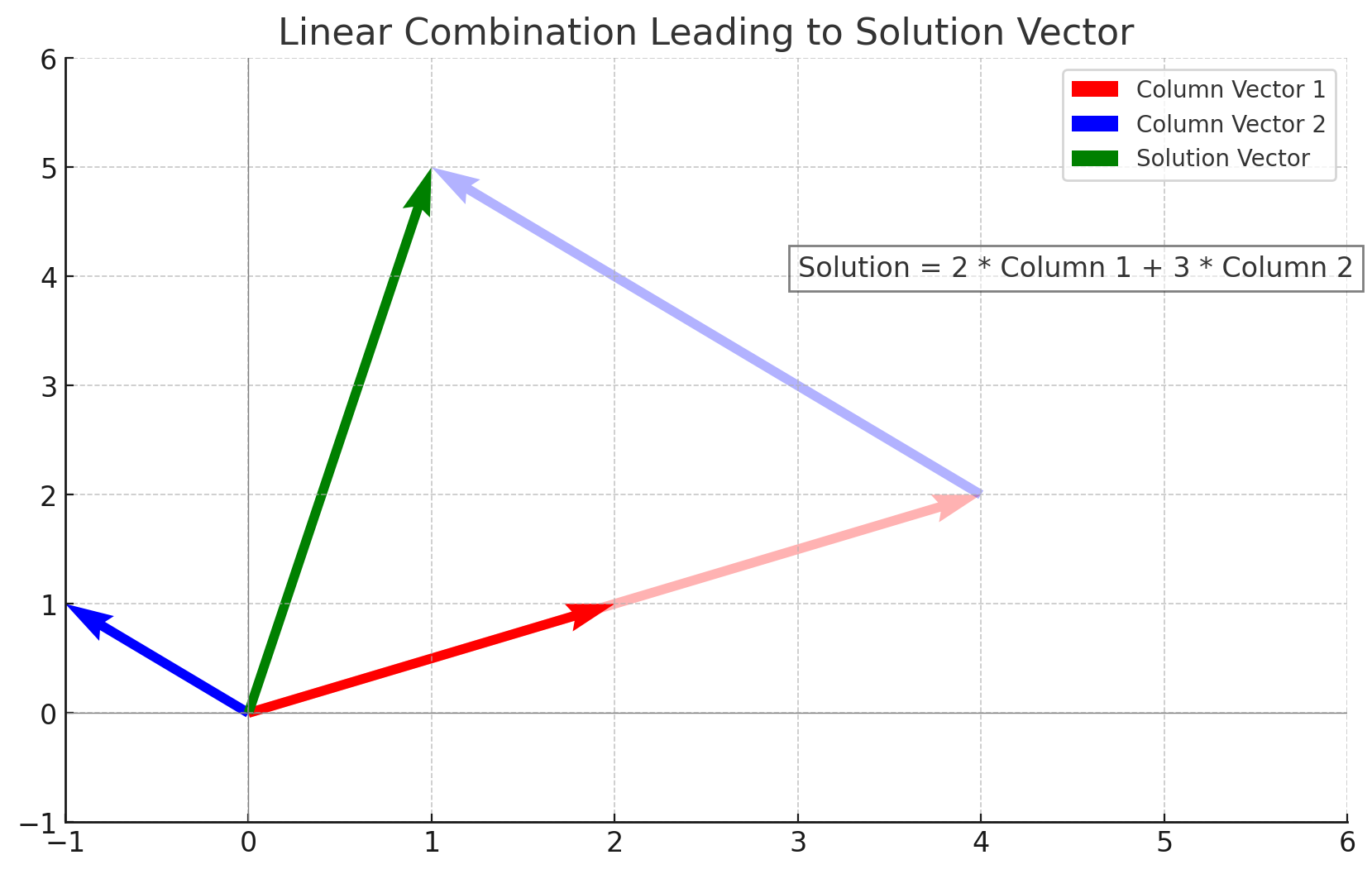
Solution to the system using column vectors. (Source: ChatGPT/matplotlib)

And indeed, the unknown coefficients turned out to be $x = 2$ and $y = 3$. So the solution to the system is indeed $\{x = 2, y = 3\}$.

Visualization in 3D

Consider these three equations:

As was the case with the previous system (where the number of dimensions was 2), there are two ways to think about these equations. The first one is the row form. Each row of these equations describes a plane in the third dimension, as opposed to just a line in the second dimension. Let’s get some geometric intuition for how that might look:

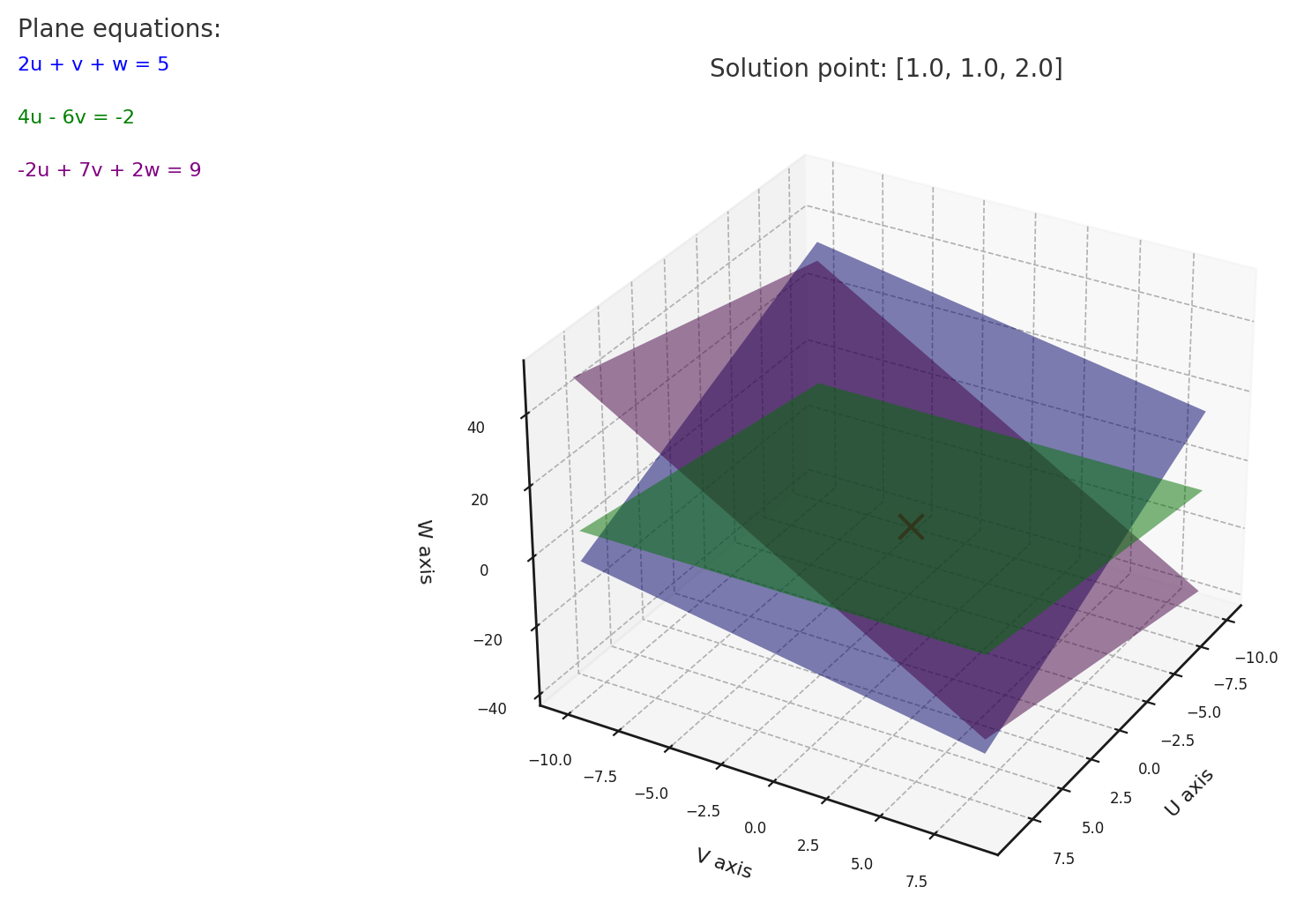
Solution to the system using planes. (Source: ChatGPT/matplotlib)

Here the three planes are plotted. Their intersection - the point $(1, 1, 2)$ - is the solution to the system.

The other way is the column form. This turns the equation into the form:

where we have to solve for the three variables $u$, $v$ and $w$. The vector $b$ is identified with the point whose coordinates are $5, -2, 9$. Let’s try solving this graphically as well. Take a look at this cool plot I (ChatGPT) made to illustrate this:

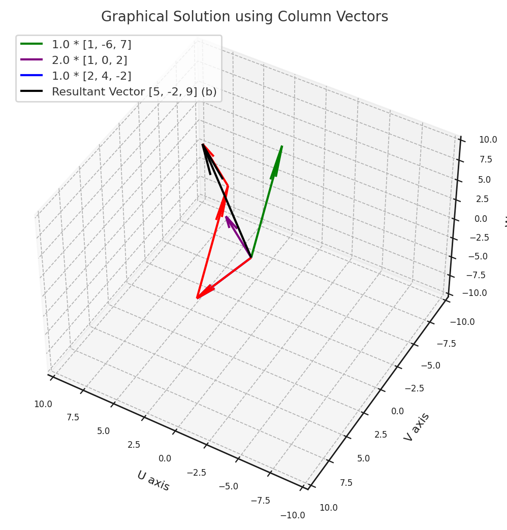
Solution to the system using vectors. (Source: ChatGPT/matplotlib)

See the coefficients of each vector? Turns out that they are the same as the coordinates of the solution point in the row form! (The blue vector is overlapping with the red one.)

This is called a linear combination of the column vectors. This linear combination is the particular one that solves the system. We have now solved the system graphically in two different manners.

Graphically speaking, when do the systems fail to have a solution? Well, simply, when the planes do not intersect. When there is no linear combination of the column vectors that results in the solution vector.