Support Vector Machines - Day 14 of ML • Juho Välimäki

Time spent: 7h
Total: 38.5h/10000h

I had to go even deeper into SVMs to properly articulate all of my knowledge into this post. This is probably my most in-depth post thus far.

Support vector machines (SVM) are an elegant and intuitive solution to classification problems. They’re a relatively new model, having their first prototype developed in 1992 at AT&T Bell Laboratories.

An Intuitive Explanation

Essentially, what SVM tries to do is find a decision boundary that separates positive and negative examples from each other. Take a look:

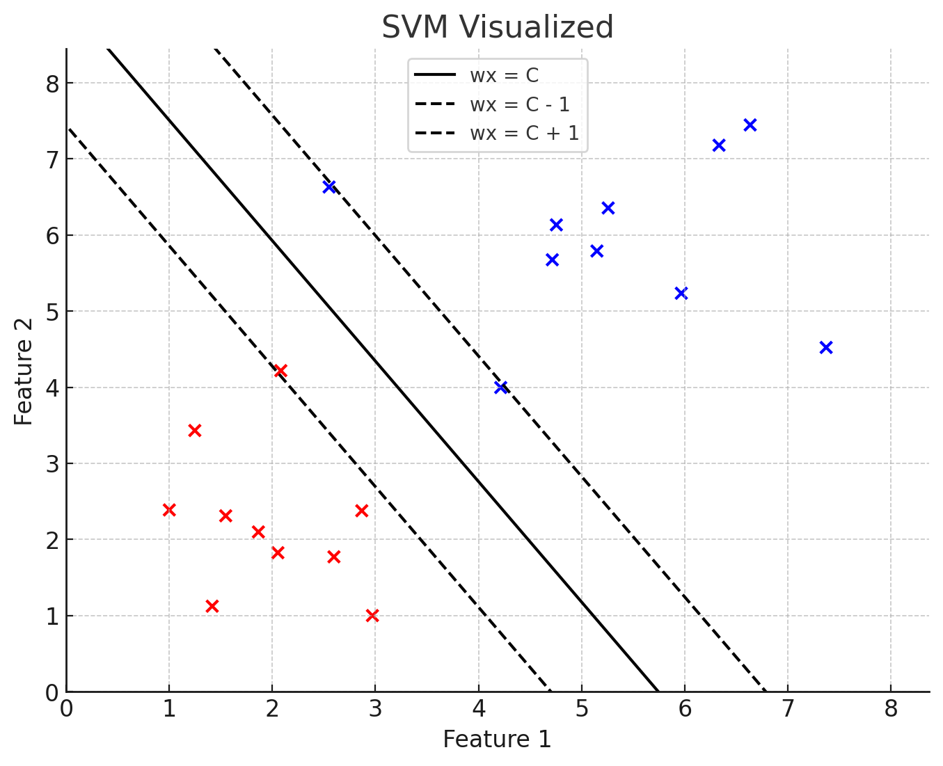
Visualization of a Support Vector Machine. (ChatGPT/matplotlib)

Here the decision boundary is the solid line in the middle. All examples below that line are negative, and all examples above it are positive. The dashed lines are called support vectors. They are identified with the data points of each class nearest to the decision boundary. The optimization problem of the SVM is to maximize the distance between the decision boundary and the nearest point. This is called the margin. It’s simply just the distance from the decision boundary to the support vectors.

The decision boundary and support vectors are not actually lines, but hyperplanes. The equation for the decision boundary is $\vec w \cdot \vec x + b = 0$ , and the equations for the upper and lower support vectors are $\vec w \cdot \vec x + b = 1$ and $\vec w \cdot \vec x + b = -1$ respectively.

However, I find it more intuitive to think of them in the form of $\vec w \cdot \vec x = c$ , where $c = -b$ . Let’s stick to this for now, and develop from here (I accidentally put a capitalized C in the graphic). This model of thinking just shifts the decision boundary away from the origin, as it isn’t there in our picture either. So maybe it’ll help.

Since our example is in 2D, we have two features $x_1$ and $x_2$ , and their corresponding weights $w_1$ and $w_2$ . Hence the equation for the decision boundary can be turned into:

\vec w \cdot \vec x = c \implies w_1x_1 + w_2x_2 = c \implies w_1x_1 + w_2x_2 + b = 0

For intuition’s sake, imagine $x_2 = y$ .

This slowly starts resembling the formula of a line $ax + by + c = 0$ :

w_1x + w_2y + b = 0

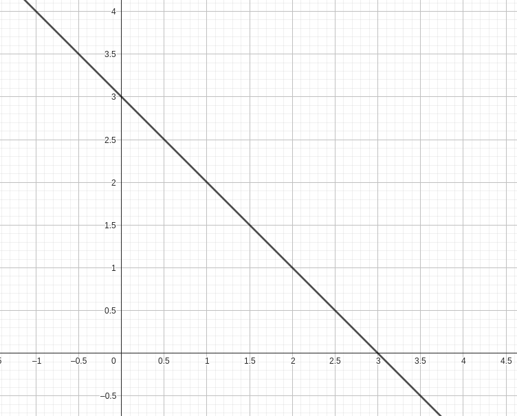
Visualization of the line x + y = 3 (or x + y - 3 = 0).

And indeed, it starts looking a bit similar as well. Anyway, the SVM just tries to measure on which side of the hyperplane the point is.

The weight vector $\vec w$ will always be orthogonal to the decision boundary (and you’ll see why later in this post), which helps to give the signed distance for how far away the data point is from the decision boundary:

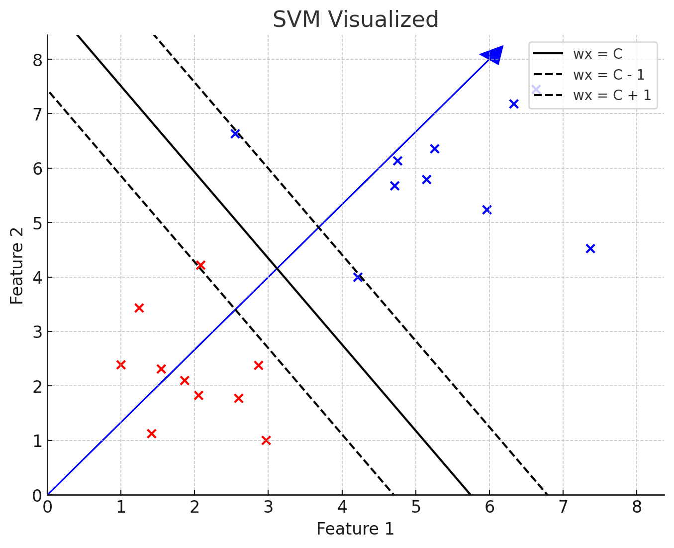
Visualization of the weight vector. (ChatGPT/matplotlib)

In reality the weight vector probably isn’t this long, this is just for illustration purposes. We’ll later on see how the weight vector actually defines the margin for the SVM.

The distance is defined as:

d(x) = \frac{\vec w \cdot \vec x + b}{||\vec w||}

where $\vec w \cdot \vec x + b$ is the value of the decision function for the SVM, and the denominator $||\vec w||$ is the norm of the weight vector. This normalizes the distance, so that the length of the weight vector doesn’t influence the value. The sign of this distance for some feature vector $\vec x$ determines whether the SVM classifies it as a positive or negative example. Let’s see how this works geometrically. Just forget the bias term $b$ for now:

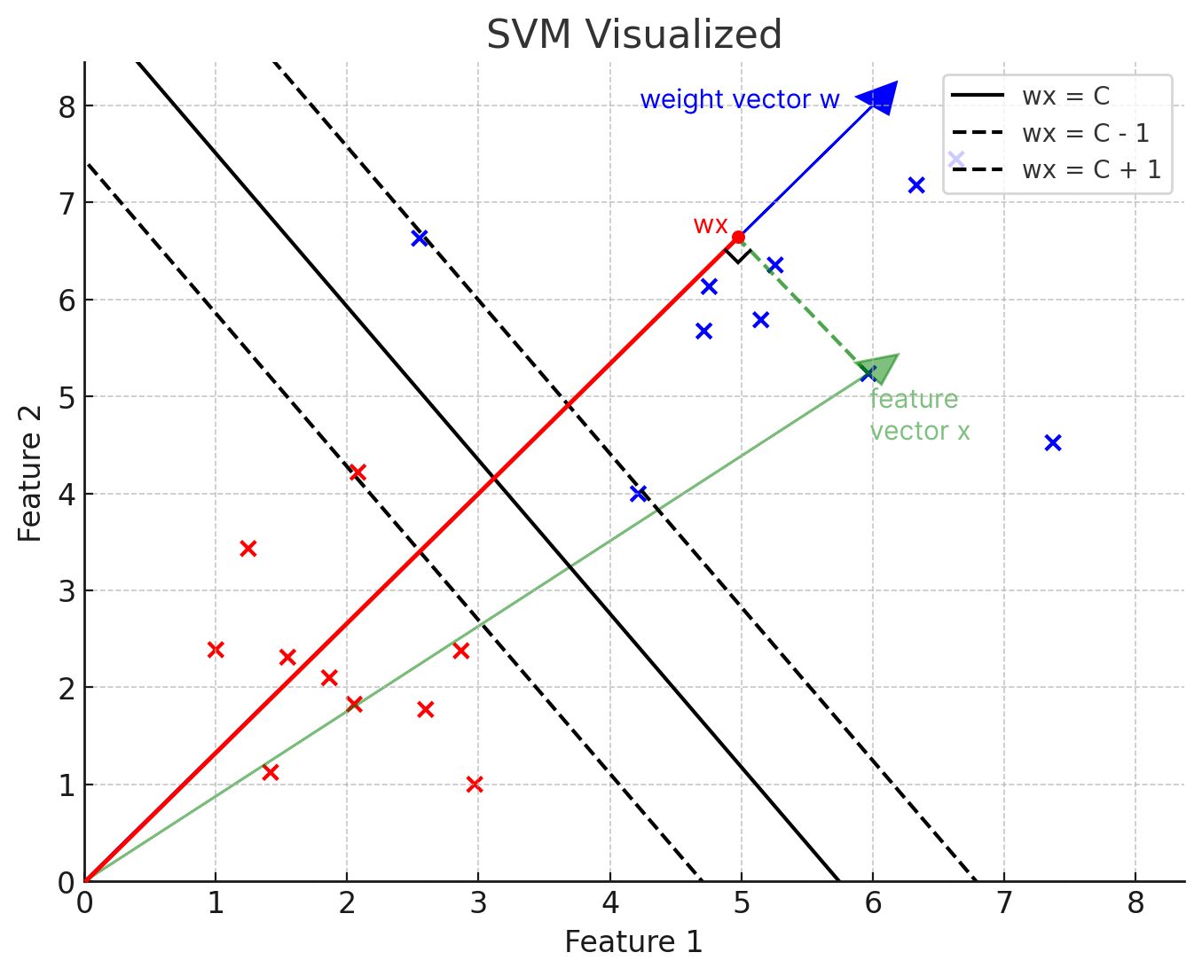
Visualization of the distance function. (ChatGPT/matplotlib)

Notice something familiar from an analytic geometry class here? The signed distance can be viewed as a projection of the vector $\vec x$ onto the vector $\vec w$ . Here we can see that the value of the distance is much more than the threshold $c$ , which is what the decision boundary requires in order for it to be classified as a positive example. And indeed, it is a positive example!

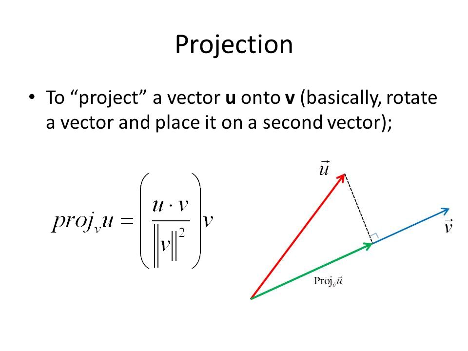
Visualization of the vector projection. (vectorified.com)

Indeed, it does look familiar.

The Mathematics

Now that we’ve developed some geometric intuition for SVMs, let’s go over the mathematical aspect to actually learn how we can implement them ourselves. For this part, forget the $c$ (which is $-b$ ) term and visualize that our decision boundary goes through the origin (since it gets shifted by there by the bias term $b$ ), $\vec w \cdot \vec x = c \implies \vec w \cdot \vec x + b = 0$ .

Also take note that it’s easy to confuse the equation for the decision boundary $\vec w \cdot \vec x + b = 0$ with the actual decision function, which is essentially just the sign of $\vec w \cdot \vec x_i + b$ .

The goal of an SVM is to find the hyperplane that maximizes the margin between the nearest data points of different classes while correctly classifying the training data points.

Let’s break this down. Let’s first take our dataset of labeled examples $S = \{(\vec x_i, y_i)\}_{i=1}^N$ .

In order for the SVM to classify all examples correctly, it must follow these two conditions:

$\vec w \cdot \vec x_i + b \leq - 1$ for all $y_-$ ,
$\vec w \cdot \vec x_i + b \geq 1$ for all $y_+$ .

These two constraints can be summarized into just one constraint: $y_i(\vec w \cdot \vec x_i + b) \geq 1$ . This effectively says that every point must be at least 1 unit away (which is the minimum margin for SVMs, by definition) from the decision boundary.

Wait, what if the dataset makes it impossible for us to have a margin that is $1$ or more whilst preserving correct classification? By definition of the SVM, the margin must always be 1 or more. However, there are two different types of SVMs:

Hard-margin SVMs, where no data points are “inside” the margins, all are strictly at least $1$ unit away from the decision boundary.
Soft-margin SVMs, where there exist data points “inside the margins”, so the distance between them and the decision boundary is less than $1$ , but the data points are still classified correctly.

For soft-margin SVMs the constraint is $y_i(\vec w \cdot \vec x_i + b) \geq 1 - \xi$ , where $\xi$ is the slack variable — or in other words the amount by which the point nearest to the decision boundary is “inside” the margin.

So the optimization problem is to maximize the margin whilst following the constraint. Let’s first look into how we get the margin. Recall this image:

Visualization of a Support Vector Machine. (ChatGPT/matplotlib)

Imagine you’re on some point on the the decision boundary $\vec w \cdot \vec x + b = 0$ (or in the image $\vec w \cdot \vec x = c$ ). To get to a point on the support vector the most direct route, we must go in the direction of the blue weight vector $w$ . So we need to go $k$ units in the direction of the unit vector of $w$ :

k \cdot \vec w^0 = k\frac{\vec w}{||\vec w||}

So as we’re standing on the decision boundary $\vec w \cdot \vec x + b = 0$ , we know that the closest point on the upper support vector is going to be $\vec w(\vec x + k\frac{\vec w}{||\vec w||}) + b = 1$ . So we need to solve for $k$ to be able to determine the distance between the two points. From there we see the distance between the decision boundary and the support vector — in other words, the margin.

This expression simplifies as follows:

\vec w(\vec x + k\frac{\vec w}{||\vec w||}) + b = 1 \implies \vec w \cdot \vec x + k\frac{\vec w \cdot \vec w}{||\vec w||} + b = 1

We know that $\vec w \cdot \vec x + b = 0$ , since we’re on the decision boundary, so we can remove those terms altogether:

k\frac{\vec w \cdot \vec w}{||\vec w||} = 1 \implies k\frac{||\vec w||^2}{||\vec w||} = 1 \implies k{||\vec w||} = 1 \implies k = \frac{1}{||w||}

So now we know how to solve for the margin. Geometrically, the distance between the two support vectors is therefore $\frac{2}{||w||}$ .

So, we need to maximize $\frac{1}{||w||}$ . How is that done? Well, by minimizing $||w||$ . However, for the sake of mathematical convenience (which you’ll see applied soon), we’ll use $\frac{1}{2}||\vec w||^2$ instead. It means the same thing.

So now the optimization problem is to find:

\min(\frac{1}{2}||\vec w||^2), \,\,\, \text{subject to} \,\,\, y_i(\vec w \cdot \vec x_i + b) \geq 1\,\,\, \forall i \in \{1..N\}

Solving The Problem With Lagrange Multipliers

It is often more convenient to solve problems of this nature with a method called Lagrange multipliers. It allows us to find the minimum value to a function whilst following a set of constraints.

In case you’re not familiar with Lagrange multipliers, I’d suggest doing some independent reading on them. I won’t be going over them in this post.

Let’s formulate the Lagrangian function $L$ :

L(\vec w, b, \vec \alpha) = \frac{1}{2}||\vec w||^2 - \sum\limits_{i=1}^n{\alpha_i[(\vec w \cdot \vec x + b) - 1]}

To get the optimal parameters $w$ and $b$ , we take the partial derivative of $L$ with respect to them and set them to 0:

\frac{\partial L}{\partial \vec w} = \vec w - \sum\limits_{i=1}^n{\alpha_iy_ix_i} = 0 \newline \frac{\partial L}{\partial b} = -\sum\limits_{i=1}^n{\alpha_iy_i} = 0

From the partial derivative we get $w = \sum\limits_{i=1}^n{\alpha_iy_ix_i}$ . Let’s substitute it back to the Lagrangian function to get the dual form:

\max\limits_{\alpha_1 \dots \alpha_N}\sum\limits_{i=1}^{N}\alpha_i - \frac{1}{2}\sum\limits_{i=1}^{N}\sum\limits_{j=1}^{N} y_i y_j \alpha_i \alpha_j (\vec x_i \cdot \vec x_j)\newline \text{subject to} \,\, \sum\limits_{i=1}^N \alpha_iy_i = 0, \,\, \,\, \alpha_i \geq 0\,\,\, \forall i \in \{1..N\}

Quite a scary expression… So, essentially we want to get the optimal values for the Lagrangian multipliers $\alpha_1 \ldots \alpha_n$ so that we maximize the expression after it. The double sum at the end accounts for the interactions between every pair of two data points by their Lagrange multipliers, labels and the dot product of their feature vectors. The other constraint comes from the partial derivative of $L$ with respect to the parameter $b$ .

The reason as to why we mess with Lagrange multipliers is because it turns the problem into a convex quadratic optimization problem. It’s going to be much more convenient for the computer to solve.

So, we get the optimal values of the Lagrange multipliers. The lagrange mutlipliers will be more than zero for the data points that are the support vectors. We use them to construct the weight vector and the support vectors, and then use the support vectors to construct the decision boundary.

So mathematically, a data point $\vec x_i$ is a support vector if and only if:

\alpha^*_i > 0

The weight vector $w$ is constructed by the support vectors:

\vec w = \sum\limits_{i=1}^N{\alpha^*_iy_i\vec x_i}

(recall the partial derivative of $L$ w.r.t $\vec w$ ) for all the points where $\alpha^*_i > 0$ .

From here we can calculate the bias vector $b$ from any of the support vectors. We know that for any support vector $(\vec x_s, y_s)$ the following must hold:

y_s(\vec w \cdot \vec x_s + b) = 1

So we can just solve for $b$ :

b = y_s - \vec w \cdot \vec x

And there we go! We have now found the optimal parameters $w$ and $b$ for the SVM.

Hyperparameters

Kernels

If our data isn’t linearly separable in the dimension we’re in, we can use a kernel trick to transform the data into the dimension above.

Let’s take the quadratic kernel as an example. Say we’re in the second dimension and we have some 2D feature vector $(a, b)$ . The quadratic kernel is simply a mapping from $(a, b)$ to $(a^2, \sqrt{2}ab, b^2)$ for all elements. Now we’re suddenly in the third dimension.

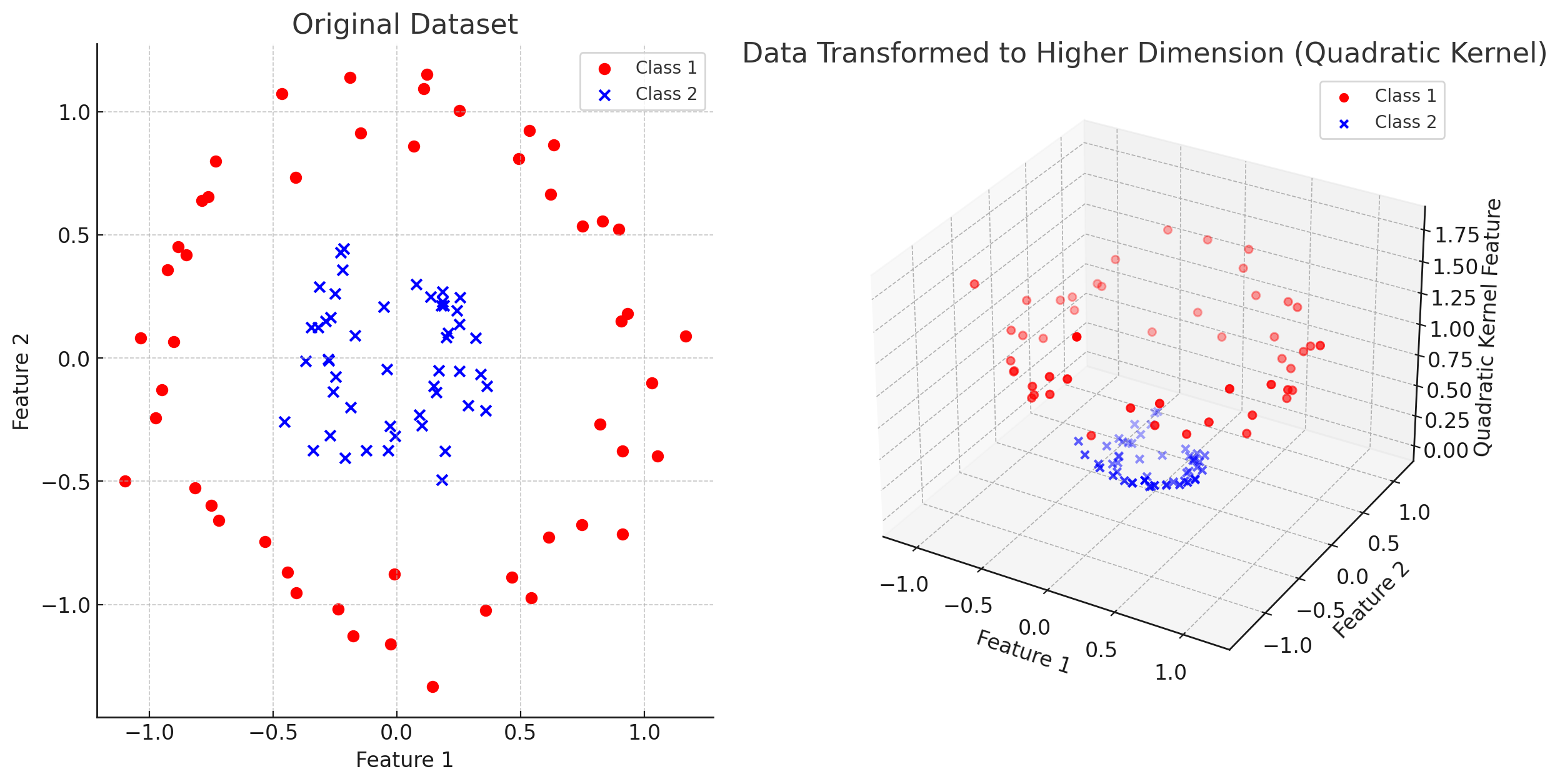
Visualization of the quadratic kernel. (ChatGPT/matplotlib)

Now our data is linearly separable by a plane. The quadratic kernel is actually used quite rarely, but it’s good for illustrating the point of kernels.

There are other kernels, the most known of which is the radial basis function (RBF) kernel.

C

$C$ is a regularization parameter that tries to balance maximizing the margin and minimizing the classification error.

A high $C$ value tries to classify every single example correctly, which may lead to worse generalization.
A low $C$ value allows for some misclassification but does that at the cost of potentially improving generaliztion.

With the regularization parameter $C$ , the optimization problem of the SVM becomes:

\min(\frac{1}{2}||\vec w||^2) + C\sum\limits_{i=1}^N{\xi_i}, \,\,\,\,\, y_i(\vec w \cdot \vec x_i + b) \geq 1 - \xi_i \,\,\,\,\, \forall i \in \{1..N\}

where again $\xi$ is the slack variable for some data point $x_i$ .

There are also other hyperparamaters for SVMs which I haven’t explored yet, but I think this will be enough for this post!