Decision Trees - Day 18 of ML • Juho Välimäki

Time spent: 4h
Total: 49h/10000h

Thus far we have only gone over parametric models. Decision trees, however, are slightly different. Instead of trying to optimize for some parameters $w, b$ , they try to form multiple optimal classification rules on the data in order to sequentially simplify a complex problem.

“A decision tree is a flowchart-like structure in which each internal node represents a “test” on an attribute (e.g. whether a coin flip comes up heads or tails), each branch represents the outcome of the test, and each leaf node represents a class label (decision taken after computing all attributes). The paths from root to leaf represent classification rules.” — Wikipedia

I think everyone studying CS has seen a structure of a tree. Decision trees look the same as any other “tree” you’d see:

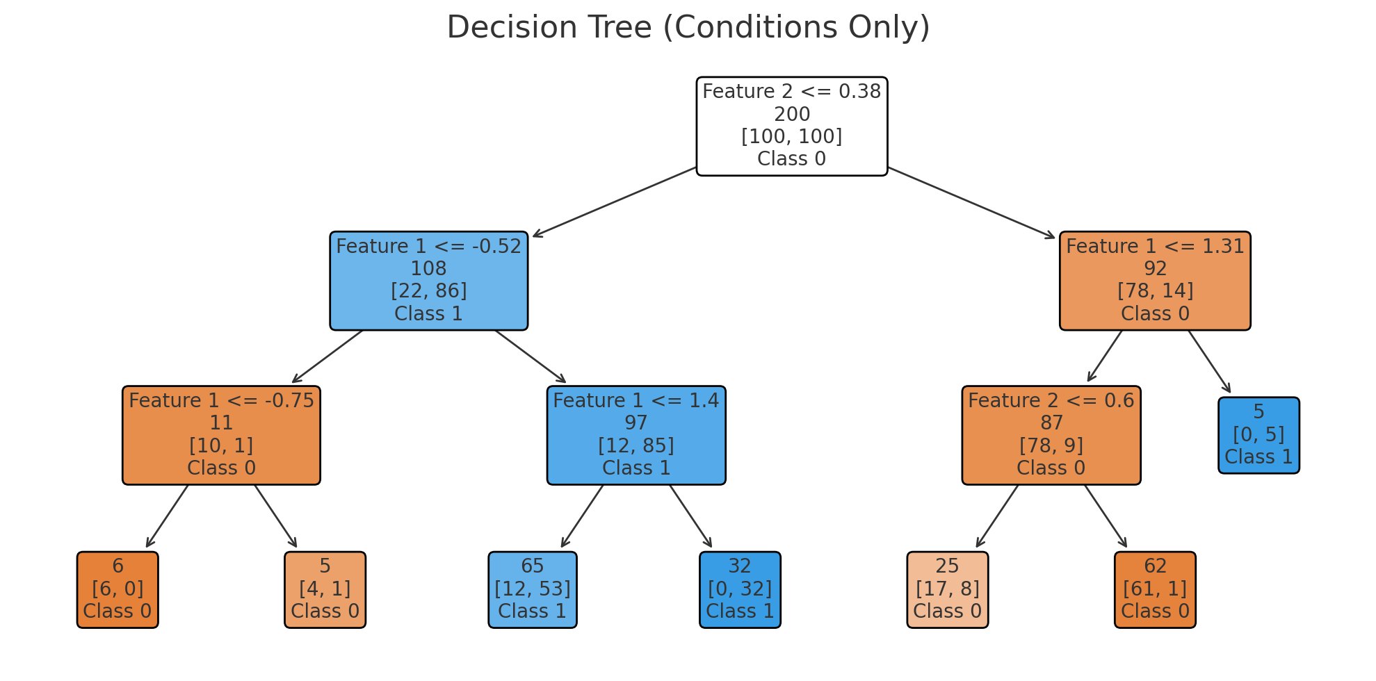
Visualization of a decision tree. (ChatGPT/matplotlib)

Let’s take the three conclusions from the Wikipedia quote:

Internal nodes represent “tests” on attributes (for example, ” $\text{Feature 2} \leq 0.38$ ”).
Each branch represents the different outcomes of a tests.
Leaf nodes represent a classification (in the example, positive examples being blue and negative ones being light brown)

The idea behind decision trees is very intuitive. Decision trees simply just apply many classification rules into the dataset. Let’s try this with an example. Consider the following dataset:

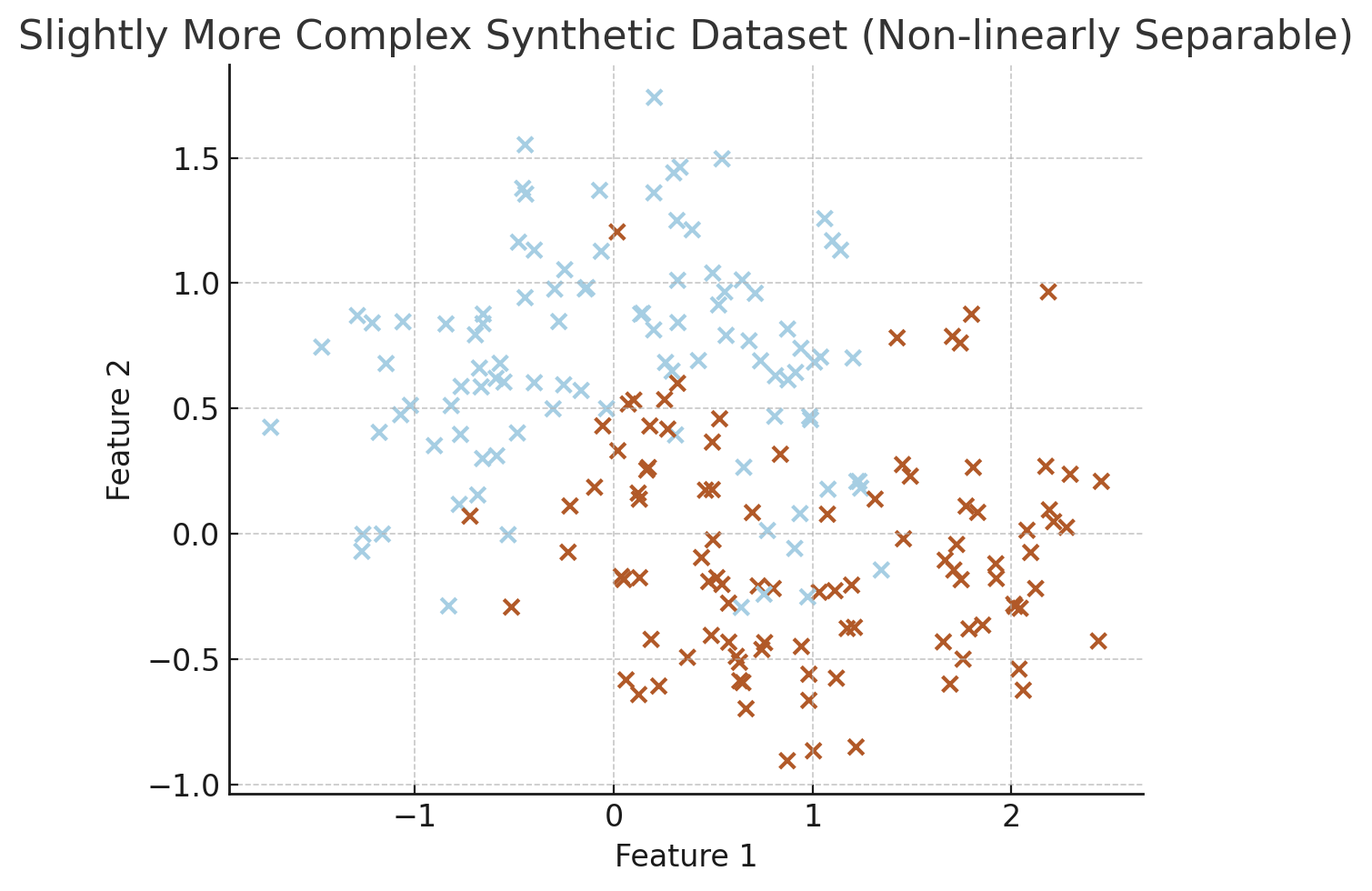
Visualization of the dataset. (ChatGPT/matplotlib)

The decision boundary is quite complex on this one. You can’t just fit a line in there. Let’s see how decision trees would solve the classification problem on this dataset:

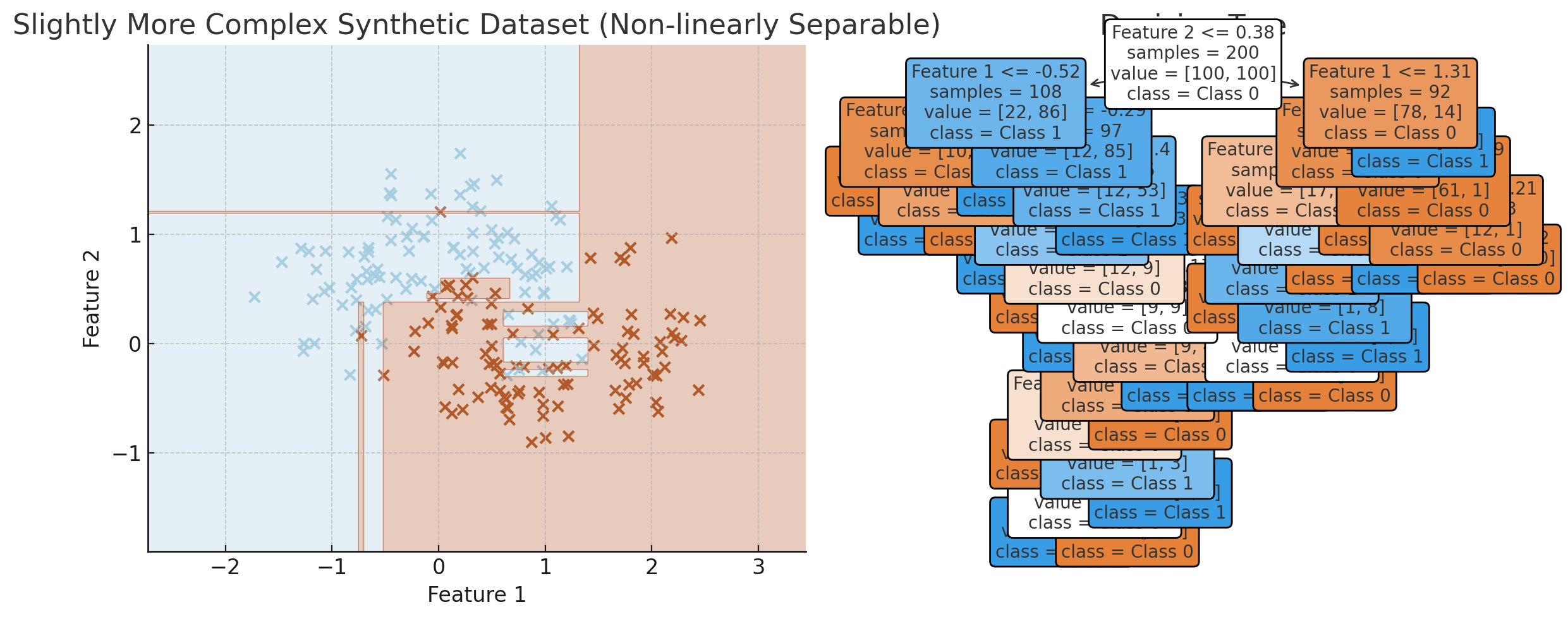
Visualization of the decision tree overfitting. (ChatGPT/matplotlib)

…yikes! That looks like overfitting to me. This decision tree would probably not generalize to new data too well. This is a centric problem with decision trees: they are prone to overfitting, especially as the depth of the tree increases. Let’s try fixing this by changing the maximum depth of the tree to $3$ :

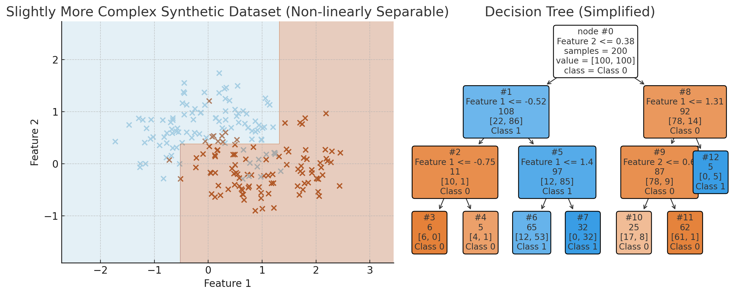
Visualization of the decision tree with depth=3. (ChatGPT/matplotlib)

That looks drastically better. The model looks like it will generalize relatively well. As you can see, every internal node does a test on some feature, and the leaf nodes represent the classification.

I feel like that’s enough for graphical intuition. I do feel like visualizing decision trees is a bit tricky in this format. I therefore left a video in the further reading section of the post — it will certainly do a better job.

Where decision trees get slightly more interesting is in how they determine the optimal classification rules. Let’s dive in to the mathematics of this.

Mathematical Prerequisites

Let’s go over some math concepts from information theory before we see how they’re applied in the model.

Entropy

Entropy is a measure of impurity/uncertainty in a dataset. Impurity? Uncertainty? Well, it measures how mixed the class labels are within a subset (for example one that is created by a classification rule of a decision tree) of data. A high impurity means that the elements in the subset belong to different classes, and a low impurity means that most or all instances belong to the same class.

The entropy $H(D)$ is defined as:

H(D) = -\sum_{i=1}^{C}{p_i \log_2(p_i)}

where:

$D$ is the dataset,
$C$ is the number of classes (in our example that would be $2$ ),
$p_i$ is the proportion of instances in class $i$ . (Proportion of instances = $\frac{\text{frequency of i}}{|D|}$ ). So $p_i$ is high if the class $i$ is common and low if it’s rare.

So why does this work? We know that since $log_2(p_i) < 0$ since $p_i \leq 1$ , so the entropy value will always be positive due to the minus sign at the beginning of the expression. The larger the proportion $p_i$ is on average, the lower the entropy value will be. Decision trees try to minimize entropy.

Information Gain

When we minimize the entropy/uncertainty, we maximize what is called the information gain.

The information gain is defined as:

\text{Information Gain}(D,A) = H(D) - \sum\limits_{v \in Values(A)}{\frac{|D_v|}{|D|} H(D_v)}

There’s a lot to go over this expression. Let’s go through it in parts:

$D$ is the entire dataset.
$A$ is the attribute/feature of the value on which we are splitting.
$Values(A)$ is the set of the possible values that the attribute/feature can have when split. Consider this: if the classification rule would be something like $A \leq 18.5$ , the decision tree will create two subsets $D_{+}$ and $D_{-}$ , where $D_+$ stands for when the threshold is met, and $D_-$ stands for when it isn’t.
$D_v$ is a subset of the dataset $D$ where the attribute $A$ has the value $v$ .
$H(D)$ and $H(D_v)$ are the entropies for the dataset and the subset, respectively.

So, we take the sum of the entropies of all the subsets after the split, and we subtract that from the entropy of the dataset. This is how we can see how much information we’d “gain” from doing the split. Decision trees try to optimize this. We try to find the most optimal point to split in order to maximize the information gain.

The ID3 Algorithm

There are many algorithms for finding the optimal decision tree for a dataset. We’ll only be looking at one since it fits the mathematical prerequisites we covered nicely. It is called the Iterative Dichotomiser 3 (ID3) algorithm.

Fortunately, since we already went over so much math, the workings of this algorithm will be quite easy to understand.

Calculate the entropy of the dataset.
Iterate over every attribute/feature in the dataset and test each threshold on them to see which one has the highest information gain.
Choose the attribute with the highest information gain, and pick a value for which the information gain is the highest.
Split the data on the picked attribute and picked value.
Repeat for every subset until one of the following holds:
- the entropy is $0$ (every element in the subset is of the same class),
- there are no more attributes to split on,
- the dataset is empty, or
- the specified maximum depth has been reached.

And that’s how you end up with a well-fit decision tree. As we saw earlier in the post, it is often useful to tweak the depth parameter of the tree to avoid overfitting.

Decision Trees - Day 18 of ML

Mathematical Prerequisites

Entropy

Information Gain

The ID3 Algorithm

Conclusion