Gradient Descent - Day 6 of ML

Time spent: 2.5h
Total: 16h/10000h

I feel like gradient descent is where ML models start to get interesting. Like, how do the models actually adapt to the data? We’ll look into that now. First, it’ll be helpful to cover a bit of math to understand the algorithm fully.

Partial Derivatives

The partial derivative of a function $f(x, y, z,...)$ with respect to some variable $x$, denoted $\frac{\partial f}{\partial x}$, is a bit like the normal derivative, just that it’s used in multivariable functions. The principle is really simple actually:

1. Assume all the other variables were constant, and
2. differentiate $f$ with respect to $x$ as if it were a single-variable function.

That’s it.

Example 1: Given $f(x) = x^2 y + y^3$, find $\frac{\partial f}{\partial x}$ and $\frac{\partial f}{\partial y}$.
Solution:

1. $\frac{\partial f}{\partial x}$: Treat $y$ as constant: $\frac{\partial}{\partial x}(x^2 y + y^3) = 2xy$.
2. $\frac{\partial f}{\partial y}$: Treat $x$ as constant: $\frac{\partial}{\partial y}{x^2 y + y^3} = x^2 + 3y^2$.

Gradient Descent

Gradient descent is a fundamental optimization algorithm used very widely in machine learning models. The point is essentially to try to minimize the value of the cost function $J$ by making small adjustments to the parameters. It uses partial derivatives under the hood to minimize $J$ using its’ gradient. Let’s look a bit into how this is done:

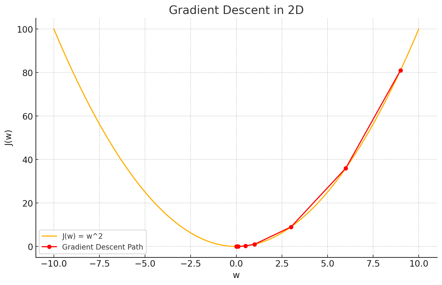
Gradient descent visualization in 2D. (ChatGPT/matplotlib)

Essentially gradient descent finds the slope of the cost function $J$, and adjusts the parameter $w$ slightly (in relation to the slope) so that the value of $J$ starts going down, step-by-step. Gradient descent requires the function to be convex — which means that the function must always be curving upwards — for example, a parabola. Note the example only has the parameter $w$ here. Let’s add a dimension and see what happens if we also add the parameter $b$:

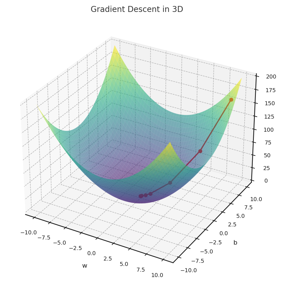
Gradient descent visualization in 3D. (ChatGPT/matplotlib)

So, the principle still says the same. It’s going to be slightly harder to visualize when we have a vector of weights, though.

Let’s take the mean squared error (MSE) cost function we went over previously. Recall:

Let’s use it in our example of linear regression, where we have features $\{x_1, x_2,\dots,x_n\}$ and weights $\{w_1, w_2,...,w_n\}$. Note we use $n$ to describe the number of features. We’ll hence use $m$ to describe the number of training examples. Now our cost function becomes

Wait. Why is it $\frac{1}{2m}$ instead of $\frac{1}{m}$? Well, the explanation is that it slightly simplifies the computation of the gradient. See, the partial derivative with respect to some parameter, let’s say $w_j$ (the weight parameter of the $j$:th feature of every training example) of the cost function when using $\frac{1}{m}$ simplifies to:

where $w_{i}^{(j)}$ is the weight for the $j$:th feature of the $i$:th training example. The notation $x^{(j)}$ is often used to describe the $j$:th feature of the input vector, and I think it makes this example a bit easier to understand. Anyway — when we divide the cost function by $\frac{1}{2m}$, it will instead simplify to

which makes it slightly nicer. That right there is the slope of the function that gradient descent tries to use to start approaching a smaller value.

Here’s roughly how the algorithmic part of gradient descent works:

1. Initialize the parameters $w$ and $b$ to some arbitrary values.
2. Compute the gradient of the cost function $J$ with respect to $w$.
3. Adjust $w$ slightly with respect to the gradient.
4. Compute the gradient of the cost function $J$ with respect to $b$.
5. Adjust $b$ slightly with respect to the gradient.
6. Repeat steps 2-5 until the value of the cost function has converged to a sufficiently small value.

Note that the parameters must be adjusted separately. You cannot compute both $w$ and $b$ first and only adjust after, since this would mess with the result.

Let’s introduce a new variable — the learning rate $\alpha$. It’s used to control how large the step of a gradient descent is, and it’s often set to some really small value, like $\alpha = 0.001$. Why is it needed? Well, see what happens when gradient descent tries to take steps too big:

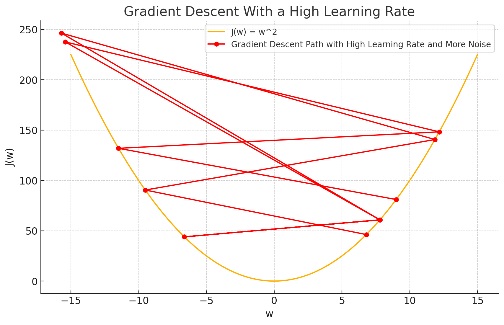
Gradient descent with a learning rate too high. (ChatGPT/matplotlib)

The function starts oscillating instead of converging nicely! It tries to jump so far that it ends up increasing the cost — drastically.

Anyway, with the learning rate, the parameter updates look like this:

Let’s implement this in code for the linear regression program we wrote earlier.

# arbitrary values
w = 1
b = -2

...

# the number of total iterations over the dataset
epochs = 100
m = len(X)

# learning rate
lr = 0.000001

for _ in range(epochs):
    w_grad = 0
    b_grad = 0
    
    # compute gradient for w
    for i in range(m):
        w_grad += (loss(w, b, X.iloc[i], Y.iloc[i])) * X.iloc[i]

    w_gradient = w_grad / m
    w -= lr * w_gradient

    # compute gradient for b
    for i in range(m):
        b_grad += (loss(w, b, X.iloc[i], Y.iloc[i]))

    b_gradient = b_grad / m
    b -= lr * b_gradient

    print(mse(w, X, b, Y))

>>>print(w, b)
1079.4370200437074 -3.825167863903606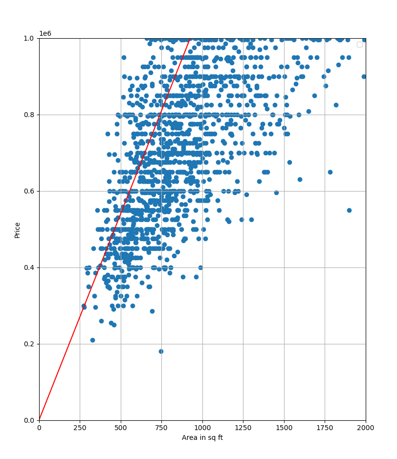

The optimal fit.

Looks like we found the optimal fit! The MSE value is still very high due to the nature of the dataset, but let’s not let that distract us. Now that I look back, a simpler dataset would’ve definitely been better to illustrate my points haha. Well, I decided to go with a real-world dataset instead.

I’ll be reimplementing gradient descent for multiple linear regression later, when I look at numpy and vectorization.