Matrices - Day 8 of ML • Juho Välimäki

Time spent: 3h
Total: 21h/10000h

If you have no prior linear algebra knowledge, I’d suggest reading yesterday’s post before reading this one. I also covered Gaussian elimination today but I didn’t write anything down about it since I found it largely uninteresting and rather trivial. I’m probably going to implement it in code eventually though.

Keeping track of all of the operations of elimination would be incredibly inconvenient with the notation we looked at previously. This is what matrix notation solves. We’ll be looking at principles of matrix multiplication as well.

Principles of Matrices

Consider the following system we were using yesterday as an example:

2u + v + w = 5\newline 4u - 6v = -2 \newline -2u + 7v + 2w = 9

What quantities do we have in this example? Well, we have:

Nine coefficients
Three unknowns $u$ , $v$ and $w$
Three right-hand sides

The right-hand side is the column vector $b$ , and on the left-hand side we have the unknowns and their coefficients. We can respresent the three unknowns as a vector:

x = \begin{bmatrix}u \\ v \\ w \end{bmatrix} = \begin{bmatrix}1 \\ 1 \\ 2\end{bmatrix}

Recall from yesterday that the solution was (1, 1, 2).

The nine coefficients form three rows and three columns. This produces a 3 by 3 coefficient matrix $\mathbf{A}$ :

\mathbf{A} = \begin{bmatrix} 2 & 1 & 1 \\ 4 & -6 & 0 \\ -2 & 7 & 2 \end{bmatrix}

$\mathbf{A}$ is a type of n by n square matrix, since the number of equations is equal to the number of unknowns. Let’s consider a case where the the number of equations is $m$ to the number of unknowns is $n$ . Then we would have an ” $m$ by $n$ matrix”.

Matrix addition works the same way as it does with vectors — one element at a time. Matrices can only be added if they have the same shape:

\begin{bmatrix} 1 & 2 \\ 3 & 4 \\ 5 & 6 \end{bmatrix} + \begin{bmatrix} 6 & 5 \\ 4 & 3 \\ 2 & 1 \end{bmatrix} = \begin{bmatrix} 1+6 & 2+5 \\ 3+4 & 4+3 \\ 5+2 & 6+1 \end{bmatrix} = \begin{bmatrix} 7 & 7 \\ 7 & 7 \\ 7 & 7 \end{bmatrix}

Multiplying matrices with a constant is equally trivial:

3 \begin{bmatrix} 1 & 2 \\ 3 & 4 \\ 5 & 6 \end{bmatrix} = \begin{bmatrix} 3 \cdot 1 & 3 \cdot 2 \\ 3 \cdot 3 & 3 \cdot 4 \\ 3 \cdot 5 & 3 \cdot 6 \end{bmatrix} = \begin{bmatrix} 3 & 6 \\ 9 & 12 \\ 15 & 18 \end{bmatrix}

Utilizing Matrices

We can represent our example system in the matrix form $Ax = b$ , where $A$ is the coefficient matrix, $x$ is the vector of unknowns, and $b$ is the solution vector:

\begin{bmatrix} 2 & 1 & 1 \\ 4 & -6 & 0 \\ -2 & 7 & 2 \end{bmatrix} \begin{bmatrix} u \\ v \\ w \end{bmatrix} = \begin{bmatrix} 5 \\ -2 \\ 9 \end{bmatrix}

To see how this kind of form works, let’s try multiplying the first row of the matrix $A$ with the vector $b$ , following the principles of matrix-vector multiplication:

\begin{bmatrix} 2 & 1 & 1 \end{bmatrix} \begin{bmatrix} u \\ v \\ w \end{bmatrix} = 2u + v + w

Just like that, we get the first equation again. It’s the same principle for the other rows as well. This is row times column multiplication. Remember the phrase row times column — it helps quite a bit when doing matrix-matrix multiplication in the future! When doing it for two vectors, it produces a single number. This is also known as the dot product or inner product of two vectors. You can also look at it as producing a 1x1 matrix:

\begin{bmatrix} 2 & 1 & 1 \end{bmatrix} \begin{bmatrix} 1 \\ 1 \\ 2 \end{bmatrix} = \begin{bmatrix}2 \cdot 1 + 1 \cdot 1 + 1 \cdot 2\end{bmatrix} = \begin{bmatrix}5\end{bmatrix}

It indeed ends up matching the first element of the solution vector! You can look at matrix-vector multiplication like that, just doing it row-by-row, or you can alternatively look at it as a combination of the three columns of $A$ :

\begin{bmatrix} 2 & 1 & 1 \\ 4 & -6 & 0 \\ -2 & 7 & 2 \end{bmatrix} \begin{bmatrix} 1 \\ 1 \\ 2 \end{bmatrix} = 1 \begin{bmatrix} 2 \\ 4 \\ -2 \end{bmatrix} + 1 \begin{bmatrix} 1 \\ -6 \\ 7 \end{bmatrix} + 2 \begin{bmatrix} 1 \\ 0 \\ 2 \end{bmatrix} = \begin{bmatrix} 5 \\ -2 \\ 9 \end{bmatrix}

Here the coefficients of each column vector are elements of $x$ . This should look familiar from yesterday’s column examples. You should also keep this way of looking at it in mind — it’s going to be important.

To be able to generalize matrix multiplications, we need a proper way to address individual elements in the matrices.

The entry in the $i$ th row and $j$ th column is denoted $a_{ij}$ . The first subscript gives the row, and the second gives the column. We can do a bit of generalization on matrix-vector multiplication with this information. The $i$ th component of $Ax$ is equal to this expression:

\sum\limits_{j=1}^{n} a_{ij}x_j

For matrix-vector multiplication, the number of columns in the matrix must be equal to the number of dimensions in the vector.

The identity matrix $I$ is a matrix with 1s on the diagonal and 0s everywhere else:

I = \begin{bmatrix} 1 & 0 & 0 \\ 0 & 1 & 0 \\ 0 & 0 & 1 \end{bmatrix}

Multiplying with the identity matrix is effectively the matrix equivalent of multiplying by 1. $Ib = b$ .

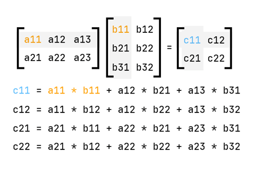
Matrix Multiplication

This is an important one. If you’re using these articles as a learning resource, definitely do research from other resources as well — especially in this case; matrix multiplication is hard for me to explain, especially by words. But I’ll leave a helpful graphic shortly.

There is only one rule/requirement involved in matrix multiplication. In order for $A$ and $B$ to be multipliable, the number of columns in $A$ has to be equal to the number of rows in $B$ . So say $A$ is of the form $m \times n$ , so $m$ rows and $n$ columns, $B$ must be of the form $n \times p$ . Just remember that rows come first — it’s always $rows \times columns$ . Sometimes it really takes a while to develop an intuition for this.

Anyway, matrix-matrix multiplication follows the same principles as matrix-vector multiplication, just that you’re now dealing with many columns in the other matrix. Otherwise, the principle stays the same — rows by columns. Let’s see this principle illustrated in this graphic:

$A GIF visualization of matrix multiplication. (Source: Tenor)$

A GIF visualization of matrix multiplication. (Source: Tenor)

So essentially,

You go to the first row on the first matrix
You multiply every column of the second matrix with that row
You go to the next row and repeat step 2.

Do a LOT of exercises on matrix multiplication, it really does take a while to get proficient at it. It’s also very prone to human error. Fortunately most of the computing is done by computer nowadays, so understanding the principle and the semantics is more important than being able to carry out all the computations yourself.

Some rules for matrix multiplication:

It is associative: $(AB)C = A(BC)$ .
It is distributive: $A(B + C) = AB + AC$ .
It is not commutative: Usually $AB \neq BA$ .